A stock option is the right to buy or sell a stock at an agreed price and date. The two types of options used for different situations are either calls, betting a stock will increase in value , or puts, betting a stock will decrease in value (however this is not always true, discussed at the end). Each options contract represents 100 shares of that stock.

There are also two different styles for options: American and European. The calculations that will be done here are for European options.

Black Scholes Model

The Black Scholes model is considered to be one of the best ways of determining fair prices of options. It requires five variables: the strike price of an option, the current stock price, the time to expiration, the risk-free rate, and the volatility.

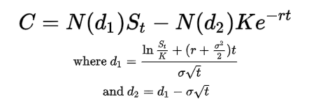
C = call option price

N = CDF of the normal distribution

St= spot price of an asset

K = strike price

r = risk-free interest rate

t = time to maturity

σ = volatility of the asset

Assumptions Made for this Calculator

It works on European options that can only be exercised at expiration.
No dividends paid out during the option’s life.
No transaction and commissions costs in buying the option.
The returns on the underlying are normally distributed.

Black Scholes in Python

For the Black Scholes formula, we need to calculate the probability of receiving the stock at the expiration of the option as well a the risk-adjusted probability that the option will be exercised. In order to do that we need a function for calculating d1 and d2. After that we could input them into a Normal distribution cumulative distribution function using scipy which will give us the probabilities. Each will require 5 inputs: S, K, T, r, and sigma.

from math import log, sqrt, pi, exp
from scipy.stats import norm
from datetime import datetime, date
import numpy as np
import pandas as pd
from pandas import DataFrame

def d1(S,K,T,r,sigma):
    return(log(S/K)+(r+sigma**2/2.)*T)/(sigma*sqrt(T))
def d2(S,K,T,r,sigma):
    return d1(S,K,T,r,sigma)-sigma*sqrt(T)

Now we could implement the Black Scholes formula in Python using the values calculated from the above functions. However, there has to be two different formulas — one for the calls, and the other for puts.

def bs_call(S,K,T,r,sigma):
    return S*norm.cdf(d1(S,K,T,r,sigma))-K*exp(-r*T)*norm.cdf(d2(S,K,T,r,sigma))

def bs_put(S,K,T,r,sigma):
    return K*exp(-r*T)-S+bs_call(S,K,T,r,sigma)

Collecting the Data

For us to test the formula on a stock we need to get the historical data for that specific stock and the other inputs related to the stock. We will be using Yahoo Finance and the pandas library to get this data.

We are able to calculate the sigma value, volatility of the stock, by multiplying the standard deviation of the stock returns over the past year by the square root of 252 (number of days the market is open over a year). As for the current price I will use the last close price in our dataset. I will also input r, the risk-free rate, as the 10-year U.S. treasury yield which you could get from ^TNX

from datetime import datetime, date
import numpy as np
import pandas as pd
import pandas_datareader.data as web

stock = 'SPY'
expiry = '12-18-2022'
strike_price = 370

today = datetime.now()
one_year_ago = today.replace(year=today.year-1)

df = web.DataReader(stock, 'yahoo', one_year_ago, today)

df = df.sort_values(by="Date")
df = df.dropna()
df = df.assign(close_day_before=df.Close.shift(1))
df['returns'] = ((df.Close - df.close_day_before)/df.close_day_before)

sigma = np.sqrt(252) * df['returns'].std()
uty = (web.DataReader(
    "^TNX", 'yahoo', today.replace(day=today.day-1), today)['Close'].iloc[-1])/100
lcp = df['Close'].iloc[-1]
t = (datetime.strptime(expiry, "%m-%d-%Y") - datetime.utcnow()).days / 365

print('The Option Price is: ', bs_call(lcp, strike_price, t, uty, sigma))

Utilizing the Function

We could now output the price of the option by using the function created before. For this example, I used a call option on ‘SPY’ with expiry ‘12–18–2020’ and a strike price of ‘370’. If all is done correctly we should get a value of approximately 16.169.

Implied Volatility and the Greeks

Some useful numbers to look at when dealing with options is the Implied Volatility. It is defined as the expected future volatility of the stock over the life of the option. It is directly influenced by the supply and demand of the underlying option and the market’s expectation of the stock price’s direction. It could be calculated by solving the Black Scholes equation backwards for the volatility starting with the option trading price.

def call_implied_volatility(Price, S, K, T, r):
    sigma = 0.001
    while sigma < 1:
        Price_implied = S * \
            norm.cdf(d1(S, K, T, r, sigma))-K*exp(-r*T) * \
            norm.cdf(d2(S, K, T, r, sigma))
        if Price-(Price_implied) < 0.001:
            return sigma
        sigma += 0.001
    return "Not Found"

def put_implied_volatility(Price, S, K, T, r):
    sigma = 0.001
    while sigma < 1:
        Price_implied = K*exp(-r*T)-S+bs_call(S, K, T, r, sigma)
        if Price-(Price_implied) < 0.001:
            return sigma
        sigma += 0.001
    return "Not Found"

print("Implied Volatility: " +
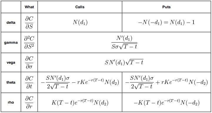
      str(100 * call_implied_volatility(bs_call(lcp, strike_price, t, uty, sigma,), lcp, strike_price, t, uty,)) + " %")

Other useful numbers people look at when dealing with options are the Greeks. The following are the main five:

Delta: the sensitivity of an option’s price changes relative to the changes in the underlying asset’s price.
Gamma: the delta’s change relative to the changes in the price of the underlying asset.
Vega: the sensitivity of an option price relative to the volatility of the underlying asset.
Theta: the sensitivity of the option price relative to the option’s time to maturity.
Rho: the sensitivity of the option price relative to interest rates.

def call_delta(S,K,T,r,sigma):
    return norm.cdf(d1(S,K,T,r,sigma))
def call_gamma(S,K,T,r,sigma):
    return norm.pdf(d1(S,K,T,r,sigma))/(S*sigma*sqrt(T))
def call_vega(S,K,T,r,sigma):
    return 0.01*(S*norm.pdf(d1(S,K,T,r,sigma))*sqrt(T))
def call_theta(S,K,T,r,sigma):
    return 0.01*(-(S*norm.pdf(d1(S,K,T,r,sigma))*sigma)/(2*sqrt(T)) - r*K*exp(-r*T)*norm.cdf(d2(S,K,T,r,sigma)))
def call_rho(S,K,T,r,sigma):
    return 0.01*(K*T*exp(-r*T)*norm.cdf(d2(S,K,T,r,sigma)))

def put_delta(S,K,T,r,sigma):
    return -norm.cdf(-d1(S,K,T,r,sigma))
def put_gamma(S,K,T,r,sigma):
    return norm.pdf(d1(S,K,T,r,sigma))/(S*sigma*sqrt(T))
def put_vega(S,K,T,r,sigma):
    return 0.01*(S*norm.pdf(d1(S,K,T,r,sigma))*sqrt(T))
def put_theta(S,K,T,r,sigma):
    return 0.01*(-(S*norm.pdf(d1(S,K,T,r,sigma))*sigma)/(2*sqrt(T)) + r*K*exp(-r*T)*norm.cdf(-d2(S,K,T,r,sigma)))
def put_rho(S,K,T,r,sigma):
    return 0.01*(-K*T*exp(-r*T)*norm.cdf(-d2(S,K,T,r,sigma)))

Options Pricing

I mentioned above that options prices are mainly affected by the prices however it is also important to know other factors that are used in their pricing. The three main shifting parameters are: the price of the underlying security, the time and the volatility. The implied volatility is key when measuring whether options prices are cheap or expensive. It allows traders to determine what they think the future volatility is likely to be. It is recommended to buy when the implied volatility is at its lowest as that generally means that their prices are discounted. This is because options that have high levels of implied volatility will result in high-priced option premiums. On the opposite side, when implied volatility is low, this means that the market’s expectations and demand for the option is decreasing, therefore causing prices to decrease.

Black Scholes Model in Python for Predicting Options Premiums

suhailsaqan