Gamma Exposure (GEX)

One of the most important parts of trading the market is finding an edge in the market which is sort of reliable to trade constantly. That usually involves when market participants like the market makers are being forced to buy or sell a certain asset.

Today we will discuss how we could use gamma exposure to come up with a somewhat consistent trading strategy. First of all, what is gamma exposure?

Gamma exposure is the second order price sensitivity of a certain derivative to changes in the price of its underlying security.

A big factor in market movements is the market makers buying and selling options from and to the traders. In order to do that they are forced to also hedge that risk they are taking by buying or selling that option’s underlying security. This process is often referred to as Delta Hedging. However, when hedging, the options value changes differently (the Delta) based off how far the underlying security’s price is from the option’s strike price. Not only the delta but also its rate of sensitivity changes as well. This rate of sensitivity is called the Gamma.

This makes the process of hedging way more complex, therefore as the price of underlying security changes the dealers would need to adjust their hedge for every point change by buying or selling additional shares in order to make sure their positions remain neutral to their side. The reason this is important to understand is because this could often cause bigger movements of volatility in the market like the recent massive movement in GameStop ($GME) share prices.

Essentially, gamma hedging could be described as the process of adjusting a delta hedge relative to the underlying security’s price. As an example, let’s say you purchased a call option with a delta of 0.50 you could hedge your long position by shorting 50 shares of the underlying security. If the option’s gamma is .10, after a 1 point increase in the security’s price the delta would become 0.6 and after the 2 point increase the gamma becomes 0.20 this would make the delta 0.80. In order to adjust to the change in Delta you would have to short 10 more shares for a 1 point increase and 20 more shares for the next. On a larger scale like the market makers and institutions, millions of shares being shorted (sold) after each point increase in the price would also affect the price of that security.

The constant force of buying or selling counter to the markets direction caused by gamma hedging is often a cause of a volatility decrease.

There are two sides to gamma hedging: long gamma or short gamma. The example I gave earlier is an example of long gamma, counter to that, short gamma is just the exact opposite. As gamma hedging causes a reverse effect on the security, for every point decrease in the price of the security the dealers would have to buy shares. By doing that, there would also be a point where the dealers would change from being overall long gamma to being short gamma or vice versa. You call this point the Zero Gamma level.

When dealers switch from being long gamma to short gamma, at the zero gamma level, that would usually cause a level of support for the securities price and therefore we see a lot of upside at that level. That is obviously due to the change from mass selling to mass buying from the dealers.

People could take advantage of this by calculating this securities zero gamma level and entering positions based off the condition from there. I will demonstrate how to calculate this using Python.

Calculating GEX and Zero Gamma Level

First of all we will be downloading data from the official Cboe website. In this example we will be using SPY but you could do it for any stock. You could find the overall code for this at the bottom.

In order to find the zero gamma exposure level we need to also find the total amount of gamma exposure for both the calls and the puts. First we will organize the data into a python data frame and store the spot price of the stock in a different variable.

We calculate the Total Gamma Exposure (GEX) for each strike by multiplying each option’s gamma, for all the calls and puts, by their respective Open Interest. After that we multiply them by 100 as the each option represents 100 shares. For the puts we multiply each by -1 as their gamma is negative. When we have them all calculated we add all the gamma with similar strikes together which would be the Total Gamma Exposure (GEX) for each strike. If you plot it it should look something like this.

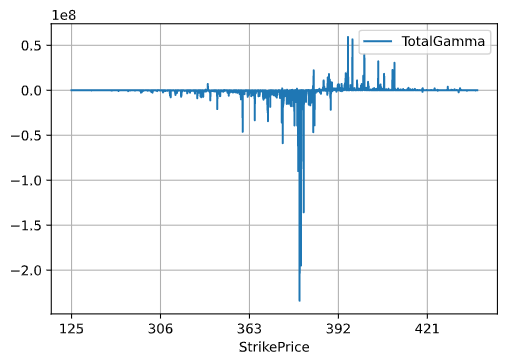
Total Gamma Exposure (GEX) vs. Strike Price

After finding that we could find the zero gamma by implementing the function I defined, zero_gex().

import pandas as pd
import numpy as np
import matplotlib.pyplot as plt
import scipy
import seaborn as sns
from datetime import timedelta, date
import datetime
from itertools import *

df = pd.read_csv('SPY-03-03', sep='\s+', header=None, skiprows=0)

df.columns = ['1stCol']

spot_price = df['1stCol'][0].split(',')[1]
spot_price = float(spot_price.split('Last:')[1])

df = df.iloc[3:]

new = df["1stCol"].str.split(",", n = 21, expand = True)
new.columns = ['ExpirationDate','Calls','CallLastSale','CallNet','CallBid','CallAsk','CallVol','CallIV','CallDelta','CallGamma','CallOpenInt','CallStrike','Puts','PutLastSale','PutNet','PutBid','PutAsk','PutVol','PutIV','PutDelta','PutGamma','PutOpenInt']

callStrike = [x[-6:-3] for x in new.Calls]
new['StrikePrice'] = callStrike

new['CallGamma'] = new['CallGamma'].astype(float)
new['CallOpenInt'] = new['CallOpenInt'].astype(float)
new['CallGEX'] = new['CallGamma'] * new['CallOpenInt'] * 100 * spot_price

new['PutGamma'] = new['PutGamma'].astype(float)
new['PutOpenInt'] = new['PutOpenInt'].astype(float)
new['PutGEX'] = new['PutGamma'] * new['PutOpenInt'] * 100 * spot_price * -1

new['TotalGamma'] = new.CallGEX + new.PutGEX
count = 0
strikeWithGamma = []
for a, b in zip(new.StrikePrice, new.TotalGamma):
    strikesPlusGamma = (a,b)
    strikeWithGamma.append(strikesPlusGamma)
new['StrikeAndGamma'] = strikeWithGamma
new = new[(new['TotalGamma'] != 0.0)]

new.sort_values('StrikePrice').plot(x = 'StrikePrice', y = 'TotalGamma', grid = True)
plt.show()

def zero_gex(strikes):
    def add(a, b):
        return (b[0], a[1] + b[1])

    cumsum = list(accumulate(strikes, add))
    if cumsum[len(strikes) // 10][1] < 0:
        op = min
    else:
        op = max
    return op(cumsum, key=lambda i: i[1])[0]

print(zero_gex(new.StrikeAndGamma))

Data file example here.

Trading the ‘Zero Gamma Level’

After finding this value on SPY, we could use it to predict bounces in the reverse direction and use that for a quick scalp trade. Another thing we could expect at the zero gamma level for SPY is a spike in VIX futures as it presents a change in risk in the market. If you are not familiar with the VIX, it is the Cboe Volatility Index which represents a real-time index of the market’s expectations for the relative strength of near-term price changes of the S&P 500 index.